Note
Go to the end to download the full example code
Understand ridge regression and cross-validation
In future examples, we will model the fMRI responses using a regularized linear regression known as ridge regression. This example explains why we use ridge regression, and how to use cross-validation to select the appropriate regularization hyper-parameter.
Linear regression is a method to model the relation between some input variables \(X \in \mathbb{R}^{(n \times p)}\) (the features) and an output variable \(y \in \mathbb{R}^{n}\) (the target). Specifically, linear regression uses a vector of coefficient \(w \in \mathbb{R}^{p}`\) to predict the output
The model is considered accurate if the predictions \(\hat{y}\) are close to the true output values \(y\). Therefore, a good linear regression model is given by the vector \(w\) that minimizes the sum of squared errors:
This is the simplest model for linear regression, and it is known as ordinary least squares (OLS).
Ordinary least squares (OLS)
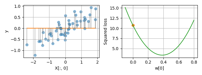
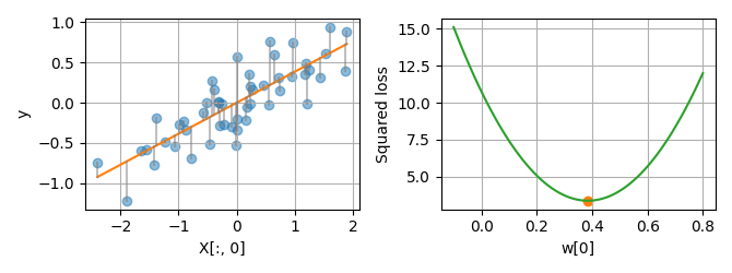
To illustrate OLS, let’s use a toy dataset with a single features X[:,0].
On the plot below (left panel), each dot is a sample (X[i,0], y[i]), and
the linear regression model is the line y = X[:,0] * w[0]. On each
sample, the error between the prediction and the true value is shown by a
gray line. By summing the squared errors over all samples, we get the squared
loss. Plotting the squared loss for every value of w leads to a parabola
(right panel).
import numpy as np
from voxelwise_tutorials.regression_toy import create_regression_toy
from voxelwise_tutorials.regression_toy import plot_1d

X, y = create_regression_toy(n_features=1)

plot_1d(X, y, w=[0])
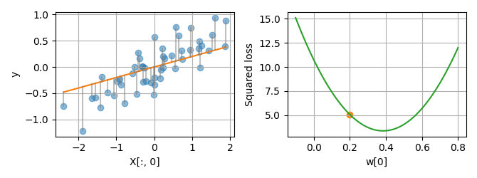
By varying the linear coefficient w, we can change the prediction
accuracy of the model, and thus the squared loss.
plot_1d(X, y, w=[0.2])
plot_1d(X, y, w=[0.7])
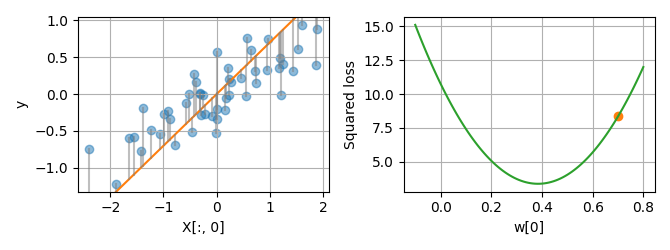
The linear coefficient leading to the minimum squared loss can be found analytically with the formula:
This is the OLS solution.
w_ols = np.linalg.solve(X.T @ X, X.T @ y)

plot_1d(X, y, w=w_ols)
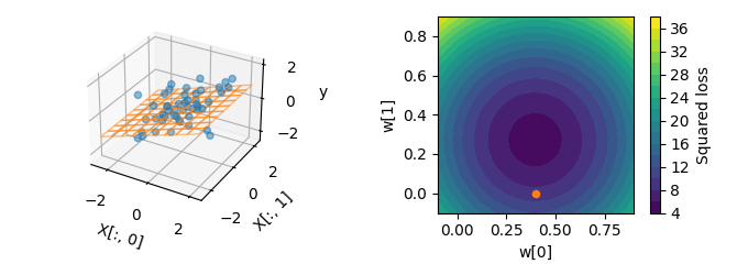
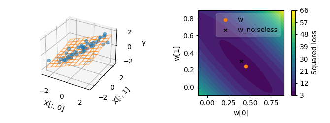
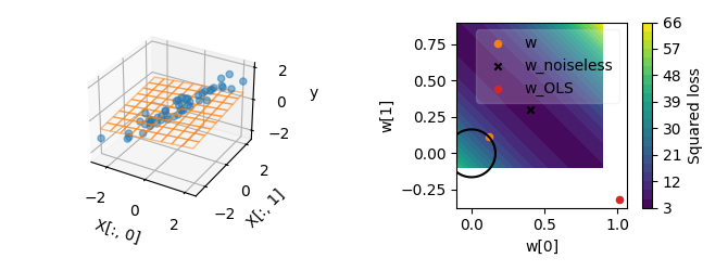
Linear regression can also be used on more than one feature. On the next toy
dataset, we will use two features X[:,0] and X[:,1]. The linear
regression model is a now plane. Here again, summing the squared errors over
all samples gives the squared loss.Plotting the squared loss for every value
of w[0] and w[1] leads to a 2D parabola (right panel).
from voxelwise_tutorials.regression_toy import create_regression_toy
from voxelwise_tutorials.regression_toy import plot_2d

X, y = create_regression_toy(n_features=2)

plot_2d(X, y, w=[0, 0], show_noiseless=False)

plot_2d(X, y, w=[0.4, 0], show_noiseless=False)
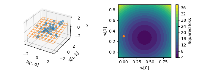
plot_2d(X, y, w=[0, 0.3], show_noiseless=False)
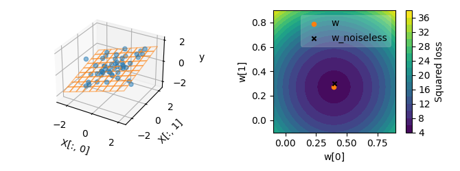
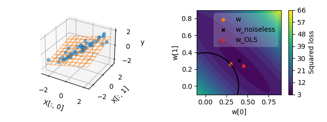
Here again, the OLS solution can be found analytically with the same formula.
Note that the OLS solution is not equal to the ground-truth coefficients used
to generate the toy dataset (black cross), because we added some noise to the
target values y. We want the solution we find to be as close as possible
to the ground-truth coefficients, because it will allow the regression to
generalize correctly to new data.
w_ols = np.linalg.solve(X.T @ X, X.T @ y)
plot_2d(X, y, w=w_ols)
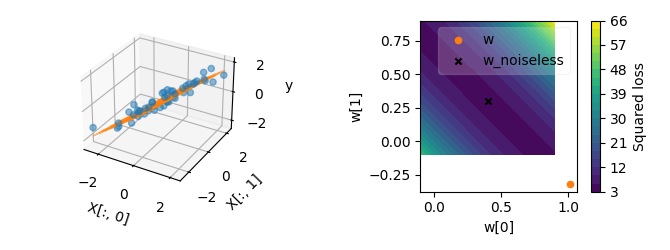
The situation becomes more interesting when the features in X are
correlated. Here, we add a correlation between the first feature X[:, 0]
and the second feature X[:, 1]. With this correlation, the squared loss
function is no more isotropic, so the lines of equal loss are now ellipses
instead of circles. Thus, when starting from the OLS solution, moving w
toward the top left leads to a small change in the loss, whereas moving it
toward the top right leads to a large change in the loss. This anisotropy
makes the OLS solution less robust to noise in some particular directions
(deviating more from the ground-truth coefficients).
X, y = create_regression_toy(n_features=2, correlation=0.9)

w_ols = np.linalg.solve(X.T @ X, X.T @ y)
plot_2d(X, y, w=w_ols)
The different robustness to noise can be understood mathematically by the fact that the OLS solution requires inverting the matrix \((X^T X)\). The matrix inversion amounts to inverting the eigenvalues \(\lambda_k\) of the matrix. When the features are highly correlated, some eigenvalues \(\lambda_k\) are close to zero, and a small change in the features can have a large effect on the inverse. Thus, having small eigenvalues reduces the stability of the inversion. If the correlation is even higher, the smallest eigenvalues get closer to zero, and the OLS solution becomes even less stable.
X, y = create_regression_toy(n_features=2, correlation=0.999)

w_ols = np.linalg.solve(X.T @ X, X.T @ y)
plot_2d(X, y, w=w_ols)
The instability can become even more pronounced with larger number of features, or with smaller numbers of samples.
X, y = create_regression_toy(n_samples=10, n_features=2, correlation=0.999)

w_ols = np.linalg.solve(X.T @ X, X.T @ y)
plot_2d(X, y, w=w_ols)
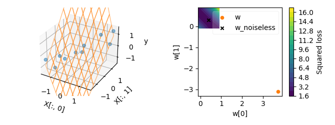
When the number of features is larger than the number of samples, the linear system becomes under-determined, which means that the OLS problem has an infinite number of solutions, most of which do not generalize well to new data.
Ridge regression
To solve the instability and under-determinacy issues of OLS, OLS can be extended to ridge regression. Ridge regression considers a different optimization problem:
This optimization problem contains two terms: (i) a data-fitting term \(||Xw - y||^2\), which ensures the regression correctly fits the training data; and (ii) a regularization term \(\alpha||w||^2\), which forces the coefficients \(w\) to be close to zero. The regularization term increases the stability of the solution, at the cost of a bias toward zero.
In the regularization term, alpha is a positive hyperparameter that
controls the regularization strength. With a smaller alpha, the solution
will be closer to the OLS solution, and with a larger alpha, the solution
will be further from the OLS solution and closer to the origin.
To illustrate this effect, the following plot shows the ridge solution for a
particular value of alpha. The black circle corresponds to the line of
equal regularization, whereas the blue ellipses are the lines of equal
squared loss.
X, y = create_regression_toy(n_features=2, correlation=0.9)

alpha = 23
w_ridge = np.linalg.solve(X.T @ X + np.eye(X.shape[1]) * alpha, X.T @ y)
plot_2d(X, y, w_ridge, alpha=alpha)
To understand why the regularization term makes the solution more robust to noise, let’s consider the ridge solution. The ridge solution can be found analytically with the formula:
where I is the identity matrix. In this formula, we can see that the
inverted matrix is now \((X^\top X + \alpha I)\). Compared to OLS, the
additional term \(\alpha I\) adds a positive value alpha to all
eigenvalues \(\lambda_k\) of \((X^\top X)\) before the matrix
inversion. Inverting \((\lambda_k + \alpha)\) instead of
\(\lambda_k\) reduces the instability caused by small eigenvalues. This
explains why the ridge solution is more robust to noise than the OLS
solution.
In the following plots, we can see that even with a stronger correlation, the ridge solution is still reasonably close to the noiseless ground truth, while the OLS solution would be far off.
X, y = create_regression_toy(n_features=2, correlation=0.999)

alpha = 23
w_ridge = np.linalg.solve(X.T @ X + np.eye(X.shape[1]) * alpha, X.T @ y)
plot_2d(X, y, w_ridge, alpha=alpha)

Changing the regularization hyperparameter \(\alpha\) leads to another ridge solution.
X, y = create_regression_toy(n_features=2, correlation=0.999)

alpha = 200
w_ridge = np.linalg.solve(X.T @ X + np.eye(X.shape[1]) * alpha, X.T @ y)
plot_2d(X, y, w_ridge, alpha=alpha)
Side note: For every \(\alpha\), at the corresponding ridge solution, the line of equal regularization and the line of equal loss are tangent. If the two lines were crossing, one could improve the ridge solution by moving along one line. It would improve one term while keeping the other term constant.
Hyperparameter selection
One issue with ridge regression is that the hyperparameter \(\alpha\) is arbitrary. Different choices of hyperparameter lead to different models. To compare these models, we cannot compare the ability to fit the training data, because the best model would just be OLS (\(alpha = 0\)). Instead, we want to compare the ability of each model to generalize to new data. To estimate a model ability to generalize, we can compute its prediction accuracy on a separate dataset that was not used during the model fitting (i.e. not used to find the coefficients \(w\)).
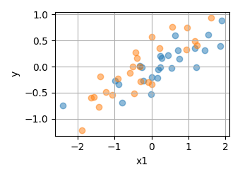
To illustrate this idea, we can split the data into two subsets.
from voxelwise_tutorials.regression_toy import create_regression_toy
from voxelwise_tutorials.regression_toy import plot_kfold2

X, y = create_regression_toy(n_features=1)

plot_kfold2(X, y, fit=False)
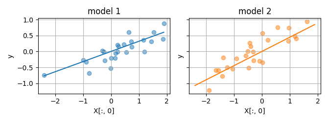
Then, we can fit a model on each subset.
alpha = 0.1
plot_kfold2(X, y, alpha, fit=True)
And compute the prediction accuracy of each model on the other subset.
plot_kfold2(X, y, alpha, fit=True, flip=True)
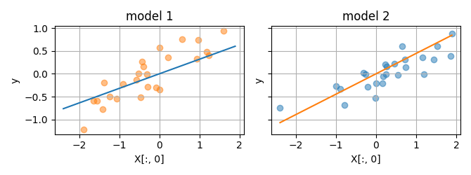
In this way, we can evaluate the ridge regression (fit with a specific \(\alpha\)) on its ability to generalize to new data. If we do that for different hyperparameter candidates \(\alpha\), we can select the model leading to the best out-of-set prediction accuracy.
from voxelwise_tutorials.regression_toy import plot_cv_path

noise = 0.1
X, y = create_regression_toy(n_features=2, noise=noise)
plot_cv_path(X, y)
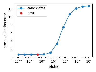
In the example above, the noise level is low, so the best hyperparameter alpha is close to zero, and ridge regression is not much better than OLS. However, if the dataset has more noise, a lower number of samples, or more correlated features, the best hyperparameter can be higher. In this case, ridge regression is better than OLS.
noise = 3
X, y = create_regression_toy(n_features=2, noise=noise)
plot_cv_path(X, y)
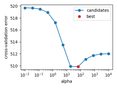
When the noise level is too high, the best hyperparameter can be the largest on the grid. It either means that the grid is too small, or that the regression does not find a predictive link between the features and the target. In this case, the model with the lowest generalization error always predict zero (\(w=0\)).
noise = 100
X, y = create_regression_toy(n_features=2, noise=noise)
plot_cv_path(X, y)
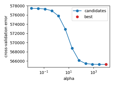
To summarize, to select the best hyperparameter \(\alpha\), the standard method is to perform a grid search:
Split the training set into two subsets: one subset used to fit the models, and one subset to estimate the prediction accuracy (validation set)
Define a number of hyperparameter candidates, for example [0.1, 1, 10, 100].
Fit a separate ridge model with each hyperparameter candidate \(\alpha\).
Compute the prediction accuracy on the validation set.
Select the hyperparameter candidate leading to the best validation accuracy.
To make the grid search less sensitive to the choice of how the training data was split, the process can be repeated for multiple splits. Then, the different prediction accuracies can be averaged over splits before the hyperparameter selection. Thus, the process is called a cross-validation.
Learn more about hyperparameter selection and cross-validation on the scikit-learn documentation.
Total running time of the script: (0 minutes 6.038 seconds)