Voxelwise modeling framework
A fundamental problem in neuroscience is to identify the information represented in different brain areas. In the VM framework, this problem is solved using encoding models. An encoding model describes how various features of the stimulus (or task) predict the activity in some part of the brain. Using VM to fit an encoding model to blood oxygen level-dependent signals (BOLD) recorded by fMRI involves several steps. First, brain activity is recorded while subjects perceive a stimulus or perform a task. Then, a set of features (that together constitute one or more feature spaces) is extracted from the stimulus or task at each point in time. For example, a video might be represented in terms of amount of motion in each part of the screen [3], or in terms of semantic categories of the objects present in the scene [4]. Each feature space corresponds to a different representation of the stimulus- or task-related information. The VM framework aims to identify if each feature space is encoded in brain activity. Each feature space thus corresponds to a hypothesis about the stimulus- or task-related information that might be represented in some part of the brain. To test this hypothesis for some specific feature space, a regression model is trained to predict brain activity from that feature space. The resulting regression model is called an encoding model. If the encoding model predicts brain activity significantly in some part of the brain, then one may conclude that some information represented in the feature space is also represented in brain activity. To maximize spatial resolution, in VM a separate encoding model is fit on each spatial sample in fMRI recordings (that is on each voxel), leading to voxelwise encoding models.
Before fitting a voxelwise encoding model, it is sometimes possible to estimate an upper bound of the model prediction accuracy in each voxel. In VM, this upper bound is called the noise ceiling, and it is related to a quantity called the explainable variance. The explainable variance quantifies the fraction of the variance in the data that is consistent across repetitions of the same stimulus. Because an encoding model makes the same predictions across repetitions of the same stimulus, the explainable variance is the fraction of the variance in the data that can be explained by the model.
To estimate the prediction accuracy of an encoding model, the model prediction is compared with the recorded brain response. However, higher-dimensional encoding models are more likely to overfit to the training data. Overfitting causes inflated prediction accuracy on the training set and poor prediction accuracy on new data. To minimize the chances of overfitting and to obtain a fair estimate of prediction accuracy, the comparison between model predictions and brain responses must be performed on a separate test data set that was not used during model training. The ability to evaluate a model on a separate test data set is a major strength of the VM framework. It provides a principled way to build complex models while limiting the amount of overfitting. To further reduce overfitting, the encoding model is regularized. In VM, regularization is obtained by ridge regression, a common and powerful regularized regression method.
To take into account the temporal delay between the stimulus and the corresponding BOLD response (i.e. the hemodynamic response), the features are duplicated multiple times using different temporal delays. The regression then estimates a separate weight for each feature and for each delay. In this way, the regression builds for each feature the best combination of temporal delays to predict brain activity. This combination of temporal delays is sometimes called a finite impulse response (FIR) filter. By estimating a separate FIR filter per feature and per voxel, VM does not assume a unique hemodynamic response function.
After fitting the regression model, the model prediction accuracy is projected on the cortical surface for visualization. Our lab created the pycortex [p3] visualization software specifically for this purpose. These prediction-accuracy maps reveal how information present in the feature space is represented across the entire cortical sheet. (Note that VM can also be applied to other brain structures, such as the cerebellum [14] and the hippocampus. However, those structures are more difficult to visualize computationally.) In an encoding model, all features are not equally useful to predict brain activity. To interpret which features are most useful to the model, VM uses the fit regression weights as a measure of relative importance of each feature. A feature with a large absolute regression weight has a large impact on the predictions, whereas a feature with a regression weight close to zero has a small impact on the predictions. Overall, the regression weight vector describes the feature tuning of a voxel, that is the feature combination that would maximally drive the voxel’s activity. To visualize these high-dimensional feature tunings over all voxels, feature tunings are projected on fewer dimensions with principal component analysis, and the first few principal components are visualized over the cortical surface [4] [8]. These feature-tuning maps reflect the selectivity of each voxel to thousands of stimulus and task features.
In VM, comparing the prediction accuracy of different feature spaces within a single data set amounts to comparing competing hypotheses about brain representations. In each brain voxel, the best-predicting feature space corresponds to the best hypothesis about the information represented in that voxel. However, many voxels represent multiple feature spaces simultaneously. To take this possibility into account, in VM a joint encoding model is fit on multiple feature spaces simultaneously. The joint model automatically combines the information from all feature spaces to maximize the joint prediction accuracy.
Because different feature spaces used in a joint model might require different regularization levels, VM uses an extended form of ridge regression that provides a separate regularization parameter for each feature space. This extension is called banded ridge regression [12]. Banded ridge regression also contains an implicit feature-space selection mechanism that tends to ignore feature spaces that are non-predictive or redundant [15]. This feature-space selection mechanism helps to disentangle correlated feature spaces and it improves generalization to new data.
To interpret the joint model, VM implements a variance decomposition method that quantifies the separate contributions of each feature space. Variance decomposition methods include variance partitioning, the split-correlation measure, or the product measure [15]. The obtained variance decomposition describes the contribution of each feature space to the joint encoding model predictions.