Note
Go to the end to download the full example code
Fit a ridge model with motion energy features
In this example, we model the fMRI responses with motion-energy features extracted from the movie stimulus. The model is a regularized linear regression model.
This tutorial reproduces part of the analysis described in Nishimoto et al (2011) [1]. See this publication for more details about the experiment, the motion-energy features, along with more results and more discussions.
Motion-energy features: Motion-energy features result from filtering a video stimulus with spatio-temporal Gabor filters. A pyramid of filters is used to compute the motion-energy features at multiple spatial and temporal scales. Motion-energy features were introduced in [1].
Summary: We first concatenate the features with multiple delays, to account for the slow hemodynamic response. A linear regression model then weights each delayed feature with a different weight, to build a predictive model of BOLD activity. Again, the linear regression is regularized to improve robustness to correlated features and to improve generalization. The optimal regularization hyperparameter is selected independently on each voxel over a grid-search with cross-validation. Finally, the model generalization performance is evaluated on a held-out test set, comparing the model predictions with the ground-truth fMRI responses.
Load the data
# path of the data directory
from voxelwise_tutorials.io import get_data_home
directory = get_data_home(dataset="vim-2")
print(directory)

# modify to use another subject
subject = "subject1"
/home/jlg/mvdoc/voxelwise_tutorials_data/vim-2
Here the data is not loaded in memory, we only take a peek at the data shape.
import os
import h5py

file_name = os.path.join(directory, f'VoxelResponses_{subject}.mat')
with h5py.File(file_name, 'r') as f:
    print(f.keys())  # Show all variables
    for key in f.keys():
        print(f[key])
<KeysViewHDF5 ['ei', 'roi', 'rt', 'rv', 'rva']>
<HDF5 group "/ei" (4 members)>
<HDF5 group "/roi" (30 members)>
<HDF5 dataset "rt": shape (73728, 7200), type "<f4">
<HDF5 dataset "rv": shape (73728, 540), type "<f4">
<HDF5 dataset "rva": shape (73728, 10, 540), type "<f4">
Then we load the fMRI responses.
import numpy as np

from voxelwise_tutorials.io import load_hdf5_array

file_name = os.path.join(directory, f'VoxelResponses_{subject}.mat')
Y_train = load_hdf5_array(file_name, key='rt')
Y_test_repeats = load_hdf5_array(file_name, key='rva')

# transpose to fit in scikit-learn's API
Y_train = Y_train.T
Y_test_repeats = np.transpose(Y_test_repeats, [1, 2, 0])

# Change to True to select only voxels from (e.g.) left V1 ("v1lh");
# Otherwise, all voxels will be modeled.
if False:
    roi = load_hdf5_array(file_name, key='/roi/v1lh').ravel()
    mask = (roi == 1)
    Y_train = Y_train[:, mask]
    Y_test_repeats = Y_test_repeats[:, :, mask]

# Z-score test runs, since the mean and scale of fMRI responses changes for
# each run. The train runs are already zscored.
Y_test_repeats -= np.mean(Y_test_repeats, axis=1, keepdims=True)
Y_test_repeats /= np.std(Y_test_repeats, axis=1, keepdims=True)

# Average test repeats, since we cannot model the non-repeatable part of
# fMRI responses.
Y_test = Y_test_repeats.mean(0)

# remove nans, mainly present on non-cortical voxels
Y_train = np.nan_to_num(Y_train)
Y_test = np.nan_to_num(Y_test)
Here we load the motion-energy features, that are going to be used for the linear regression model.
file_name = os.path.join(directory, "features", "motion_energy.hdf")
X_train = load_hdf5_array(file_name, key='X_train')
X_test = load_hdf5_array(file_name, key='X_test')

# We use single precision float to speed up model fitting on GPU.
X_train = X_train.astype("float32")
X_test = X_test.astype("float32")
Define the cross-validation scheme
To select the best hyperparameter through cross-validation, we must define a train-validation splitting scheme. Since fMRI time-series are autocorrelated in time, we should preserve as much as possible the time blocks. In other words, since consecutive time samples are correlated, we should not put one time sample in the training set and the immediately following time sample in the validation set. Thus, we define here a leave-one-run-out cross-validation split, which preserves each recording run.
from sklearn.model_selection import check_cv
from voxelwise_tutorials.utils import generate_leave_one_run_out

n_samples_train = X_train.shape[0]

# indice of first sample of each run, each run having 600 samples
run_onsets = np.arange(0, n_samples_train, 600)

# define a cross-validation splitter, compatible with scikit-learn
cv = generate_leave_one_run_out(n_samples_train, run_onsets)
cv = check_cv(cv)  # copy the splitter into a reusable list
Define the model
Now, let’s define the model pipeline.
from sklearn.pipeline import make_pipeline
from sklearn.preprocessing import StandardScaler

# Display the scikit-learn pipeline with an HTML diagram.
from sklearn import set_config
set_config(display='diagram')  # requires scikit-learn 0.23
With one target, we could directly use the pipeline in scikit-learn’s GridSearchCV, to select the optimal hyperparameters over cross-validation. However, GridSearchCV can only optimize one score. Thus, in the multiple target case, GridSearchCV can only optimize e.g. the mean score over targets. Here, we want to find a different optimal hyperparameter per target/voxel, so we use himalaya’s KernelRidgeCV instead.
from himalaya.kernel_ridge import KernelRidgeCV
We first concatenate the features with multiple delays, to account for the hemodynamic response. The linear regression model will then weight each delayed feature with a different weight, to build a predictive model.
With a sample every 1 second, we use 8 delays [1, 2, 3, 4, 5, 6, 7, 8] to cover the most part of the hemodynamic response peak.
from voxelwise_tutorials.delayer import Delayer
The package``himalaya`` implements different computational backends, including GPU backends. The available GPU backends are “torch_cuda” and “cupy”. (These backends are only available if you installed the corresponding package with CUDA enabled. Check the pytorch/cupy documentation for install instructions.)
Here we use the “torch_cuda” backend, but if the import fails we continue with the default “numpy” backend. The “numpy” backend is expected to be slower since it only uses the CPU.
from himalaya.backend import set_backend
backend = set_backend("torch_cuda", on_error="warn")
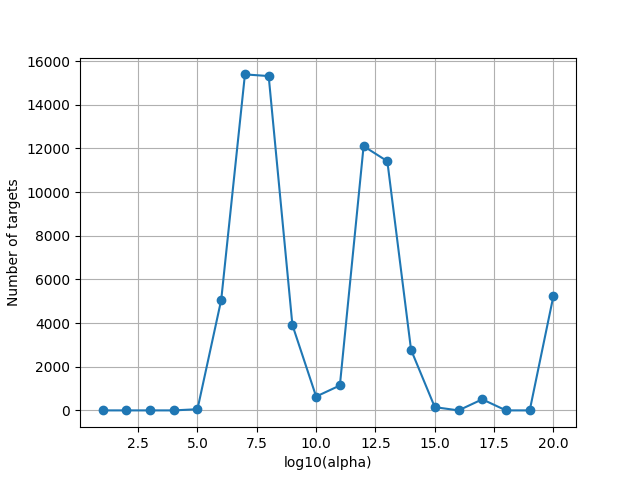
The scale of the regularization hyperparameter alpha is unknown, so we use a large logarithmic range, and we will check after the fit that best hyperparameters are not all on one range edge.
alphas = np.logspace(1, 20, 20)
The scikit-learn Pipeline can be used as a regular estimator, calling pipeline.fit, pipeline.predict, etc. Using a pipeline can be useful to clarify the different steps, avoid cross-validation mistakes, or automatically cache intermediate results.
pipeline = make_pipeline(
    StandardScaler(with_mean=True, with_std=False),
    Delayer(delays=[1, 2, 3, 4, 5, 6, 7, 8]),
    KernelRidgeCV(
        alphas=alphas, cv=cv,
        solver_params=dict(n_targets_batch=100, n_alphas_batch=2,
                           n_targets_batch_refit=50),
        Y_in_cpu=True),
)
pipeline
Fit the model
We fit on the train set, and score on the test set.
pipeline.fit(X_train, Y_train)

scores = pipeline.score(X_test, Y_test)
# Since we performed the KernelRidgeCV on GPU, scores are returned as
# torch.Tensor on GPU. Thus, we need to move them into numpy arrays on CPU, to
# be able to use them e.g. in a matplotlib figure.
scores = backend.to_numpy(scores)
Since the scale of alphas is unknown, we plot the optimal alphas selected by the solver over cross-validation. This plot is helpful to refine the alpha grid if the range is too small or too large.
Note that some voxels are at the maximum regularization of the grid. These are voxels where the model has no predictive power, and where the optimal regularization is large to lead to a prediction equal to zero.
import matplotlib.pyplot as plt
from himalaya.viz import plot_alphas_diagnostic

plot_alphas_diagnostic(best_alphas=backend.to_numpy(pipeline[-1].best_alphas_),
                       alphas=alphas)
plt.show()
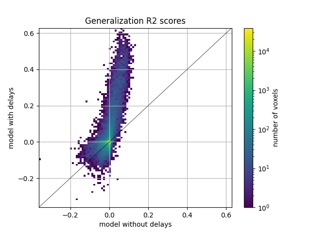
Compare with a model without delays
To present an example of model comparison, we define here another model, without feature delays (i.e. no Delayer). This model is unlikely to perform well, since fMRI responses are delayed in time with respect to the stimulus.
pipeline = make_pipeline(
    StandardScaler(with_mean=True, with_std=False),
    KernelRidgeCV(
        alphas=alphas, cv=cv,
        solver_params=dict(n_targets_batch=100, n_alphas_batch=2,
                           n_targets_batch_refit=50),
        Y_in_cpu=True),
)
pipeline
pipeline.fit(X_train, Y_train)
scores_nodelay = pipeline.score(X_test, Y_test)
scores_nodelay = backend.to_numpy(scores_nodelay)
/home/jlg/mvdoc/miniconda3/envs/voxelwise_tutorials/lib/python3.10/site-packages/himalaya/kernel_ridge/_sklearn_api.py:490: UserWarning: Solving linear kernel ridge is slower than solving ridge when n_samples > n_features (here 7200 > 6555). Using himalaya.ridge.RidgeCV would be faster. Use warn=False to silence this warning.
  warnings.warn(
Here we plot the comparison of model performances with a 2D histogram. All ~70k voxels are represented in this histogram, where the diagonal corresponds to identical performance for both models. A distribution deviating from the diagonal means that one model has better predictive performances than the other.
from voxelwise_tutorials.viz import plot_hist2d

ax = plot_hist2d(scores_nodelay, scores)
ax.set(title='Generalization R2 scores', xlabel='model without delays',
       ylabel='model with delays')
plt.show()
References
Total running time of the script: (7 minutes 12.384 seconds)