Note
Go to the end to download the full example code
Fit a ridge model with wordnet features
In this example, we model the fMRI responses with semantic “wordnet” features, manually annotated on each frame of the movie stimulus. The model is a regularized linear regression model, known as ridge regression. Since this model is used to predict brain activity from the stimulus, it is called a (voxelwise) encoding model.
This example reproduces part of the analysis described in Huth et al (2012) [1]. See this publication for more details about the experiment, the wordnet features, along with more results and more discussions.
Wordnet features: The features used in this example are semantic labels manually annotated on each frame of the movie stimulus. The semantic labels include nouns (such as “woman”, “car”, or “building”) and verbs (such as “talking”, “touching”, or “walking”), for a total of 1705 distinct category labels. To interpret our model, labels can be organized in a graph of semantic relationship based on the Wordnet dataset.
Summary: We first concatenate the features with multiple temporal delays to account for the slow hemodynamic response. We then use linear regression to fit a predictive model of brain activity. The linear regression is regularized to improve robustness to correlated features and to improve generalization performance. The optimal regularization hyperparameter is selected over a grid-search with cross-validation. Finally, the model generalization performance is evaluated on a held-out test set, comparing the model predictions to the corresponding ground-truth fMRI responses.
Path of the data directory
from voxelwise_tutorials.io import get_data_home
directory = get_data_home(dataset="shortclips")
print(directory)
/home/jlg/mvdoc/voxelwise_tutorials_data/shortclips
# modify to use another subject
subject = "S01"
Load the data
We first load the fMRI responses. These responses have been preprocessed as
described in [1]. The data is separated into a training set Y_train and a
testing set Y_test. The training set is used for fitting models, and
selecting the best models and hyperparameters. The test set is later used
to estimate the generalization performance of the selected model. The
test set contains multiple repetitions of the same experiment to estimate
an upper bound of the model prediction accuracy (cf. previous example).
import os
import numpy as np
from voxelwise_tutorials.io import load_hdf5_array

file_name = os.path.join(directory, "responses", f"{subject}_responses.hdf")
Y_train = load_hdf5_array(file_name, key="Y_train")
Y_test = load_hdf5_array(file_name, key="Y_test")

print("(n_samples_train, n_voxels) =", Y_train.shape)
print("(n_repeats, n_samples_test, n_voxels) =", Y_test.shape)
(n_samples_train, n_voxels) = (3600, 84038)
(n_repeats, n_samples_test, n_voxels) = (10, 270, 84038)
If we repeat an experiment multiple times, part of the fMRI responses might change. However the modeling features do not change over the repeats, so the voxelwise encoding model will predict the same signal for each repeat. To have an upper bound of the model prediction accuracy, we keep only the repeatable part of the signal by averaging the test repeats.
Y_test = Y_test.mean(0)

print("(n_samples_test, n_voxels) =", Y_test.shape)
(n_samples_test, n_voxels) = (270, 84038)
We fill potential NaN (not-a-number) values with zeros.
Y_train = np.nan_to_num(Y_train)
Y_test = np.nan_to_num(Y_test)
Then, we load the semantic “wordnet” features, extracted from the stimulus at
each time point. The features corresponding to the training set are noted
X_train, and the features corresponding to the test set are noted
X_test.
feature_space = "wordnet"

file_name = os.path.join(directory, "features", f"{feature_space}.hdf")
X_train = load_hdf5_array(file_name, key="X_train")
X_test = load_hdf5_array(file_name, key="X_test")

print("(n_samples_train, n_features) =", X_train.shape)
print("(n_samples_test, n_features) =", X_test.shape)
(n_samples_train, n_features) = (3600, 1705)
(n_samples_test, n_features) = (270, 1705)
Define the cross-validation scheme
To select the best hyperparameter through cross-validation, we must define a cross-validation splitting scheme. Because fMRI time-series are autocorrelated in time, we should preserve as much as possible the temporal correlation. In other words, because consecutive time samples are correlated, we should not put one time sample in the training set and the immediately following time sample in the validation set. Thus, we define here a leave-one-run-out cross-validation split that keeps each recording run intact.
from sklearn.model_selection import check_cv
from voxelwise_tutorials.utils import generate_leave_one_run_out

# indice of first sample of each run
run_onsets = load_hdf5_array(file_name, key="run_onsets")
print(run_onsets)
[ 0 300 600 900 1200 1500 1800 2100 2400 2700 3000 3300]
We define a cross-validation splitter, compatible with scikit-learn API.
n_samples_train = X_train.shape[0]
cv = generate_leave_one_run_out(n_samples_train, run_onsets)
cv = check_cv(cv)  # copy the cross-validation splitter into a reusable list
Define the model
Now, let’s define the model pipeline.
We first center the features, since we will not use an intercept. The mean value in fMRI recording is non-informative, so each run is detrended and demeaned independently, and we do not need to predict an intercept value in the linear model.
However, we prefer to avoid normalizing by the standard deviation of each feature. If the features are extracted in a consistent way from the stimulus, their relative scale is meaningful. Normalizing them independently from each other would remove this information. Moreover, the wordnet features are one-hot-encoded, which means that each feature is either present (1) or not present (0) in each sample. Normalizing one-hot-encoded features is not recommended, since it would scale disproportionately the infrequent features.
from sklearn.preprocessing import StandardScaler
scaler = StandardScaler(with_mean=True, with_std=False)
Then we concatenate the features with multiple delays to account for the hemodynamic response. Due to neurovascular coupling, the recorded BOLD signal is delayed in time with respect to the stimulus onset. With different delayed versions of the features, the linear regression model will weigh each delayed feature with a different weight to maximize the predictions. With a sample every 2 seconds, we typically use 4 delays [1, 2, 3, 4] to cover the hemodynamic response peak. In the next example, we further describe this hemodynamic response estimation.
from voxelwise_tutorials.delayer import Delayer
delayer = Delayer(delays=[1, 2, 3, 4])
Finally, we use a ridge regression model. Ridge regression is a linear
regression with L2 regularization. The L2 regularization improves robustness
to correlated features and improves generalization performance. The L2
regularization is controlled by a hyperparameter alpha that needs to be
tuned for each dataset. This regularization hyperparameter is usually
selected over a grid search with cross-validation, selecting the
hyperparameter that maximizes the predictive performances on the validation
set. See the previous example for more details about ridge regression and
hyperparameter selection.
For computational reasons, when the number of features is larger than the number of samples, it is more efficient to solve ridge regression using the (equivalent) dual formulation [2]. This dual formulation is equivalent to kernel ridge regression with a linear kernel. Here, we have 3600 training samples, and 1705 * 4 = 6820 features (we multiply by 4 since we use 4 time delays), therefore it is more efficient to use kernel ridge regression.
With one target, we could directly use the pipeline in scikit-learn’s
GridSearchCV, to select the optimal regularization hyperparameter
(alpha) over cross-validation. However, GridSearchCV can only
optimize a single score across all voxels (targets). Thus, in the
multiple-target case, GridSearchCV can only optimize (for example) the
mean score over targets. Here, we want to find a different optimal
hyperparameter per target/voxel, so we use the package himalaya which implements a
scikit-learn compatible estimator KernelRidgeCV, with hyperparameter
selection independently on each target.
from himalaya.kernel_ridge import KernelRidgeCV
himalaya implements different computational backends,
including two backends that use GPU for faster computations. The two
available GPU backends are “torch_cuda” and “cupy”. (Each backend is only
available if you installed the corresponding package with CUDA enabled. Check
the pytorch/cupy documentation for install instructions.)
Here we use the “torch_cuda” backend, but if the import fails we continue with the default “numpy” backend. The “numpy” backend is expected to be slower since it only uses the CPU.
from himalaya.backend import set_backend
backend = set_backend("torch_cuda", on_error="warn")
print(backend)
<module 'himalaya.backend.torch_cuda' from '/home/jlg/mvdoc/miniconda3/envs/voxelwise_tutorials/lib/python3.10/site-packages/himalaya/backend/torch_cuda.py'>
To speed up model fitting on GPU, we use single precision float numbers. (This step probably does not change significantly the performances on non-GPU backends.)
X_train = X_train.astype("float32")
X_test = X_test.astype("float32")
Since the scale of the regularization hyperparameter alpha is unknown, we
use a large logarithmic range, and we will check after the fit that best
hyperparameters are not all on one range edge.
alphas = np.logspace(1, 20, 20)
We also indicate some batch sizes to limit the GPU memory.
kernel_ridge_cv = KernelRidgeCV(
    alphas=alphas, cv=cv,
    solver_params=dict(n_targets_batch=500, n_alphas_batch=5,
                       n_targets_batch_refit=100))
Finally, we use a scikit-learn Pipeline to link the different steps
together. A Pipeline can be used as a regular estimator, calling
pipeline.fit, pipeline.predict, etc. Using a Pipeline can be
useful to clarify the different steps, avoid cross-validation mistakes, or
automatically cache intermediate results. See the scikit-learn
documentation for
more information.
from sklearn.pipeline import make_pipeline
pipeline = make_pipeline(
    scaler,
    delayer,
    kernel_ridge_cv,
)
We can display the scikit-learn pipeline with an HTML diagram.
from sklearn import set_config
set_config(display='diagram')  # requires scikit-learn 0.23
pipeline
Fit the model
We fit on the training set..
_ = pipeline.fit(X_train, Y_train)
..and score on the test set. Here the scores are the \(R^2\) scores, with values in \(]-\infty, 1]\). A value of \(1\) means the predictions are perfect.
Note that since himalaya is implementing multiple-targets
models, the score method differs from scikit-learn API and returns
one score per target/voxel.
scores = pipeline.score(X_test, Y_test)
print("(n_voxels,) =", scores.shape)
(n_voxels,) = torch.Size([84038])
If we fit the model on GPU, scores are returned on GPU using an array object
specific to the backend we used (such as a torch.Tensor). Thus, we need to
move them into numpy arrays on CPU, to be able to use them for example in
a matplotlib figure.
scores = backend.to_numpy(scores)
Plot the model prediction accuracy
To visualize the model prediction accuracy, we can plot it for each voxel on a flattened surface of the brain. To do so, we use a mapper that is specific to the each subject’s brain. (Check previous example to see how to use the mapper to Freesurfer average surface.)
import matplotlib.pyplot as plt
from voxelwise_tutorials.viz import plot_flatmap_from_mapper

mapper_file = os.path.join(directory, "mappers", f"{subject}_mappers.hdf")
ax = plot_flatmap_from_mapper(scores, mapper_file, vmin=0, vmax=0.4)
plt.show()
We can see that the “wordnet” features successfully predict part of the measured brain activity, with \(R^2\) scores as high as 0.4. Note that these scores are generalization scores, since they are computed on a test set that was not used during model fitting. Since we fitted a model independently in each voxel, we can inspect the generalization performances at the best available spatial resolution: individual voxels.
The best-predicted voxels are located in visual semantic areas like EBA, or FFA. This is expected since the wordnet features encode semantic information about the visual stimulus. For more discussions about these results, we refer the reader to the original publication [1].
Plot the selected hyperparameters
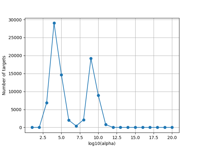
Since the scale of alphas is unknown, we plot the optimal alphas selected by the solver over cross-validation. This plot is helpful to refine the alpha grid if the range is too small or too large.
Note that some voxels might be at the maximum regularization value in the grid search. These are voxels where the model has no predictive power, thus the optimal regularization parameter is large to lead to a prediction equal to zero. We do not need to extend the alpha range for these voxels.
from himalaya.viz import plot_alphas_diagnostic
best_alphas = backend.to_numpy(pipeline[-1].best_alphas_)
plot_alphas_diagnostic(best_alphas=best_alphas, alphas=alphas)
plt.show()
Visualize the regression coefficients
Here, we go back to the main model on all voxels. Since our model is linear, we can use the (primal) regression coefficients to interpret the model. The basic intuition is that the model will use larger coefficients on features that have more predictive power.
Since we know the meaning of each feature, we can interpret the large regression coefficients. In the case of wordnet features, we can even build a graph that represents the features that are linked by a semantic relationship.
We first get the (primal) ridge regression coefficients from the fitted model.
primal_coef = pipeline[-1].get_primal_coef()
primal_coef = backend.to_numpy(primal_coef)
print("(n_delays * n_features, n_voxels) =", primal_coef.shape)
(n_delays * n_features, n_voxels) = (6820, 84038)
Because the ridge model allows a different regularization per voxel, the regression coefficients may have very different scales. In turn, these different scales can introduce a bias in the interpretation, focusing the attention disproportionately on voxels fitted with the lowest alpha. To address this issue, we rescale the regression coefficient to have a norm equal to the square-root of the \(R^2\) scores. We found empirically that this rescaling best matches results obtained with a regularization shared across voxels. This rescaling also removes the need to select only best performing voxels, because voxels with low prediction accuracies are rescaled to have a low norm.
primal_coef /= np.linalg.norm(primal_coef, axis=0)[None]
primal_coef *= np.sqrt(np.maximum(0, scores))[None]
Then, we aggregate the coefficients across the different delays.
# split the ridge coefficients per delays
delayer = pipeline.named_steps['delayer']
primal_coef_per_delay = delayer.reshape_by_delays(primal_coef, axis=0)
print("(n_delays, n_features, n_voxels) =", primal_coef_per_delay.shape)
del primal_coef

# average over delays
average_coef = np.mean(primal_coef_per_delay, axis=0)
print("(n_features, n_voxels) =", average_coef.shape)
del primal_coef_per_delay
(n_delays, n_features, n_voxels) = (4, 1705, 84038)
(n_features, n_voxels) = (1705, 84038)
Even after averaging over delays, the coefficient matrix is still too large to interpret it. Therefore, we use principal component analysis (PCA) to reduce the dimensionality of the matrix.
from sklearn.decomposition import PCA

pca = PCA(n_components=4)
pca.fit(average_coef.T)
components = pca.components_
print("(n_components, n_features) =", components.shape)
(n_components, n_features) = (4, 1705)
We can check the ratio of explained variance by each principal component. We see that the first four components already explain a large part of the coefficients variance.
print("PCA explained variance =", pca.explained_variance_ratio_)
PCA explained variance = [0.35199594 0.08103119 0.05653881 0.03766727]
Similarly to [1], we correct the coefficients of features linked by a semantic relationship. When building the wordnet features, if a frame was labeled with wolf, the authors automatically added the semantically linked categories canine, carnivore, placental mammal, mamma, vertebrate, chordate, organism, and whole. The authors thus argue that the same correction needs to be done on the coefficients.
from voxelwise_tutorials.wordnet import load_wordnet
from voxelwise_tutorials.wordnet import correct_coefficients
_, wordnet_categories = load_wordnet(directory=directory)
components = correct_coefficients(components.T, wordnet_categories).T
components -= components.mean(axis=1)[:, None]
components /= components.std(axis=1)[:, None]
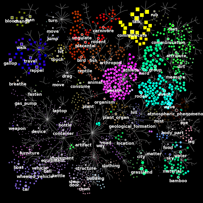
Finally, we plot the first principal component on the wordnet graph. In such graph, edges indicate “is a” relationships (e.g. an athlete “is a” person). Each marker represents a single noun (circle) or verb (square). The area of each marker indicates the principal component magnitude, and the color indicates the sign (red is positive, blue is negative).
from voxelwise_tutorials.wordnet import plot_wordnet_graph
from voxelwise_tutorials.wordnet import apply_cmap

first_component = components[0]
node_sizes = np.abs(first_component)
node_colors = apply_cmap(first_component, vmin=-2, vmax=2, cmap='coolwarm',
                         n_colors=2)

plot_wordnet_graph(node_colors=node_colors, node_sizes=node_sizes)
plt.show()
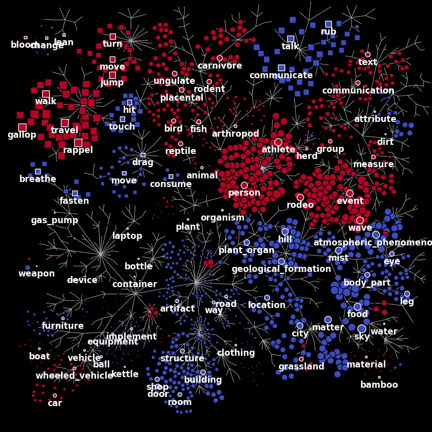
According to the authors of [1], “this principal component distinguishes between categories with high stimulus energy (e.g. moving objects like person and vehicle) and those with low stimulus energy (e.g. stationary objects like sky and city)”.
In this example, because we use only a single subject and we perform a different voxel selection, our result is slightly different than in the original publication. We also use a different regularization parameter in each voxel, while in [1] all voxels had the same regularization parameter. However, we do not aim at reproducing exactly the results of the original publication, but we rather describe the general approach.
To project the principal component on the cortical surface, we first need to use the fitted PCA to transform the primal weights of all voxels.
# transform with the fitted PCA
average_coef_transformed = pca.transform(average_coef.T).T
print("(n_components, n_voxels) =", average_coef_transformed.shape)
del average_coef

# We make sure vmin = -vmax, so that the colormap is centered on 0.
vmax = np.percentile(np.abs(average_coef_transformed), 99.9)

# plot the primal weights projected on the first principal component.
ax = plot_flatmap_from_mapper(average_coef_transformed[0], mapper_file,
                              vmin=-vmax, vmax=vmax, cmap='coolwarm')
plt.show()
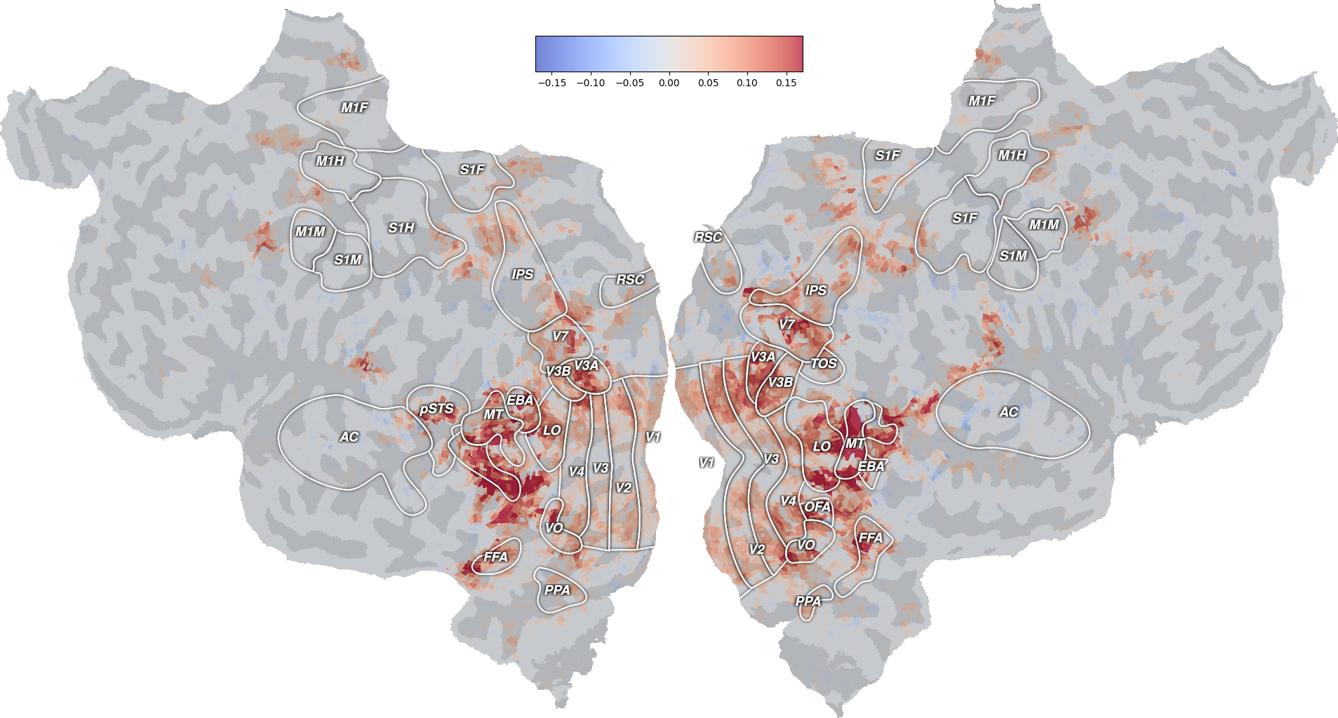
(n_components, n_voxels) = (4, 84038)
This flatmap shows in which brain regions the model has the largest projection on the first component. Again, this result is different from the one in [1], and should only be considered as reproducing the general approach.
Following [1], we also plot the next three principal components on the wordnet graph, mapping the three vectors to RGB colors.
from voxelwise_tutorials.wordnet import scale_to_rgb_cube

next_three_components = components[1:4].T
node_sizes = np.linalg.norm(next_three_components, axis=1)
node_colors = scale_to_rgb_cube(next_three_components)
print("(n_nodes, n_channels) =", node_colors.shape)

plot_wordnet_graph(node_colors=node_colors, node_sizes=node_sizes)
plt.show()
(n_nodes, n_channels) = (1705, 3)
According to the authors of [1], “this graph shows that categories thought to be semantically related (e.g. athletes and walking) are represented similarly in the brain”.
Finally, we project these principal components on the cortical surface.
from voxelwise_tutorials.viz import plot_3d_flatmap_from_mapper

voxel_colors = scale_to_rgb_cube(average_coef_transformed[1:4].T, clip=3).T
print("(n_channels, n_voxels) =", voxel_colors.shape)

ax = plot_3d_flatmap_from_mapper(voxel_colors[0], voxel_colors[1],
                                 voxel_colors[2], mapper_file=mapper_file,
                                 vmin=0, vmax=1, vmin2=0, vmax2=1, vmin3=0,
                                 vmax3=1)
plt.show()
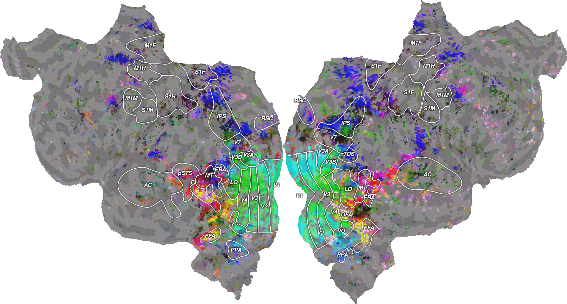
(n_channels, n_voxels) = (3, 84038)
Again, our results are different from the ones in [1], for the same reasons mentioned earlier.
References
Total running time of the script: (1 minutes 16.347 seconds)