Note
Go to the end to download the full example code
Fit a banded ridge model with both wordnet and motion energy features
In this example, we model the fMRI responses with a banded ridge regression, with two different feature spaces: motion energy and wordnet categories.
Banded ridge regression: Since the relative scaling of both feature spaces is unknown, we use two regularization hyperparameters (one per feature space) in a model called banded ridge regression [1]. Just like with ridge regression, we optimize the hyperparameters over cross-validation. An efficient implementation of this model is available in the himalaya package.
Running time: This example is more computationally intensive than the previous examples. With a GPU backend, model fitting takes around 6 minutes. With a CPU backend, it can last 10 times more.
Path of the data directory
from voxelwise_tutorials.io import get_data_home
directory = get_data_home(dataset="shortclips")
print(directory)
/home/jlg/mvdoc/voxelwise_tutorials_data/shortclips
# modify to use another subject
subject = "S01"
Load the data
As in the previous examples, we first load the fMRI responses, which are our regression targets.
import os
import numpy as np
from voxelwise_tutorials.io import load_hdf5_array

file_name = os.path.join(directory, "responses", f"{subject}_responses.hdf")
Y_train = load_hdf5_array(file_name, key="Y_train")
Y_test = load_hdf5_array(file_name, key="Y_test")

print("(n_samples_train, n_voxels) =", Y_train.shape)
print("(n_repeats, n_samples_test, n_voxels) =", Y_test.shape)
(n_samples_train, n_voxels) = (3600, 84038)
(n_repeats, n_samples_test, n_voxels) = (10, 270, 84038)
We also compute the explainable variance, to exclude voxels with low explainable variance from the fit, and speed up the model fitting.
from voxelwise_tutorials.utils import explainable_variance
ev = explainable_variance(Y_test)
print("(n_voxels,) =", ev.shape)

mask = ev > 0.1
print("(n_voxels_mask,) =", ev[mask].shape)
(n_voxels,) = (84038,)
(n_voxels_mask,) = (6849,)
We average the test repeats, to remove the non-repeatable part of fMRI responses.
Y_test = Y_test.mean(0)

print("(n_samples_test, n_voxels) =", Y_test.shape)
(n_samples_test, n_voxels) = (270, 84038)
We fill potential NaN (not-a-number) values with zeros.
Y_train = np.nan_to_num(Y_train)
Y_test = np.nan_to_num(Y_test)
And we make sure the targets are centered.
Y_train -= Y_train.mean(0)
Y_test -= Y_test.mean(0)
Then we load both feature spaces, that are going to be used for the linear regression model.
feature_names = ["wordnet", "motion_energy"]

Xs_train = []
Xs_test = []
n_features_list = []
for feature_space in feature_names:
    file_name = os.path.join(directory, "features", f"{feature_space}.hdf")
    Xi_train = load_hdf5_array(file_name, key="X_train")
    Xi_test = load_hdf5_array(file_name, key="X_test")

    Xs_train.append(Xi_train.astype(dtype="float32"))
    Xs_test.append(Xi_test.astype(dtype="float32"))
    n_features_list.append(Xi_train.shape[1])

# concatenate the feature spaces
X_train = np.concatenate(Xs_train, 1)
X_test = np.concatenate(Xs_test, 1)

print("(n_samples_train, n_features_total) =", X_train.shape)
print("(n_samples_test, n_features_total) =", X_test.shape)
print("[n_features_wordnet, n_features_motion_energy] =", n_features_list)
(n_samples_train, n_features_total) = (3600, 8260)
(n_samples_test, n_features_total) = (270, 8260)
[n_features_wordnet, n_features_motion_energy] = [1705, 6555]
Define the cross-validation scheme
We define again a leave-one-run-out cross-validation split scheme.
from sklearn.model_selection import check_cv
from voxelwise_tutorials.utils import generate_leave_one_run_out

# indice of first sample of each run
run_onsets = load_hdf5_array(file_name, key="run_onsets")
print(run_onsets)
[ 0 300 600 900 1200 1500 1800 2100 2400 2700 3000 3300]
We define a cross-validation splitter, compatible with scikit-learn API.
n_samples_train = X_train.shape[0]
cv = generate_leave_one_run_out(n_samples_train, run_onsets)
cv = check_cv(cv)  # copy the cross-validation splitter into a reusable list
Define the model
The model pipeline contains similar steps than the pipeline from previous
examples. We remove the mean of each feature with a StandardScaler,
and add delays with a Delayer.
from sklearn.pipeline import make_pipeline
from sklearn.preprocessing import StandardScaler
from voxelwise_tutorials.delayer import Delayer
from himalaya.backend import set_backend
backend = set_backend("torch_cuda", on_error="warn")
To fit the banded ridge model, we use himalaya’s
MultipleKernelRidgeCV model, with a separate linear kernel per feature
space. Similarly to KernelRidgeCV, the model optimizes the
hyperparameters over cross-validation. However, while KernelRidgeCV has
to optimize only one hyperparameter (alpha), MultipleKernelRidgeCV
has to optimize m hyperparameters, where m is the number of feature
spaces (here m = 2). To do so, the model implements two different
solvers, one using hyperparameter random search, and one using hyperparameter
gradient descent. For large number of targets, we recommend using the
random-search solver.
The class takes a number of common parameters during initialization, such as
kernels, or solver. Since the solver parameters vary depending on the
solver used, they are passed as a solver_params dictionary.
from himalaya.kernel_ridge import MultipleKernelRidgeCV

# Here we will use the "random_search" solver.
solver = "random_search"

# We can check its specific parameters in the function docstring:
solver_function = MultipleKernelRidgeCV.ALL_SOLVERS[solver]
print("Docstring of the function %s:" % solver_function.__name__)
print(solver_function.__doc__)
Docstring of the function solve_multiple_kernel_ridge_random_search:
Solve multiple kernel ridge regression using random search.

    Parameters
    ----------
    Ks : array of shape (n_kernels, n_samples, n_samples)
        Input kernels.
    Y : array of shape (n_samples, n_targets)
        Target data.
    n_iter : int, or array of shape (n_iter, n_kernels)
        Number of kernel weights combination to search.
        If an array is given, the solver uses it as the list of kernel weights
        to try, instead of sampling from a Dirichlet distribution. Examples:
          - `n_iter=np.eye(n_kernels)` implement a winner-take-all strategy
            over kernels.
          - `n_iter=np.ones((1, n_kernels))/n_kernels` solves a (standard)
            kernel ridge regression.
    concentration : float, or list of float
        Concentration parameters of the Dirichlet distribution.
        If a list, iteratively cycle through the list.
        Not used if n_iter is an array.
    alphas : float or array of shape (n_alphas, )
        Range of ridge regularization parameter.
    score_func : callable
        Function used to compute the score of predictions versus Y.
    cv : int or scikit-learn splitter
        Cross-validation splitter. If an int, KFold is used.
    fit_intercept : boolean
        Whether to fit an intercept. If False, Ks should be centered
        (see KernelCenterer), and Y must be zero-mean over samples.
        Only available if return_weights == 'dual'.
    return_weights : None, 'primal', or 'dual'
        Whether to refit on the entire dataset and return the weights.
    Xs : array of shape (n_kernels, n_samples, n_features) or None
        Necessary if return_weights == 'primal'.
    local_alpha : bool
        If True, alphas are selected per target, else shared over all targets.
    jitter_alphas : bool
        If True, alphas range is slightly jittered for each gamma.
    random_state : int, or None
        Random generator seed. Use an int for deterministic search.
    n_targets_batch : int or None
        Size of the batch for over targets during cross-validation.
        Used for memory reasons. If None, uses all n_targets at once.
    n_targets_batch_refit : int or None
        Size of the batch for over targets during refit.
        Used for memory reasons. If None, uses all n_targets at once.
    n_alphas_batch : int or None
        Size of the batch for over alphas. Used for memory reasons.
        If None, uses all n_alphas at once.
    progress_bar : bool
        If True, display a progress bar over gammas.
    Ks_in_cpu : bool
        If True, keep Ks in CPU memory to limit GPU memory (slower).
        This feature is not available through the scikit-learn API.
    conservative : bool
        If True, when selecting the hyperparameter alpha, take the largest one
        that is less than one standard deviation away from the best.
        If False, take the best.
    Y_in_cpu : bool
        If True, keep the target values ``Y`` in CPU memory (slower).
    diagonalize_method : str in {"eigh", "svd"}
        Method used to diagonalize the kernel.
    return_alphas : bool
        If True, return the best alpha value for each target.

    Returns
    -------
    deltas : array of shape (n_kernels, n_targets)
        Best log kernel weights for each target.
    refit_weights : array or None
        Refit regression weights on the entire dataset, using selected best
        hyperparameters. Refit weights are always stored on CPU memory.
        If return_weights == 'primal', shape is (n_features, n_targets),
        if return_weights == 'dual', shape is (n_samples, n_targets),
        else, None.
    cv_scores : array of shape (n_iter, n_targets)
        Cross-validation scores per iteration, averaged over splits, for the
        best alpha. Cross-validation scores will always be on CPU memory.
    best_alphas : array of shape (n_targets, )
        Best alpha value per target. Only returned if return_alphas is True.
    intercept : array of shape (n_targets,)
        Intercept. Only returned when fit_intercept is True.
The hyperparameter random-search solver separates the hyperparameters into a
shared regularization alpha and a vector of positive kernel weights which
sum to one. This separation of hyperparameters allows to explore efficiently
a large grid of values for alpha for each sampled kernel weights vector.
We use 20 random-search iterations to have a reasonably fast example. To have better results, especially for larger number of feature spaces, one might need more iterations. (Note that there is currently no stopping criterion in the random-search method.)
n_iter = 20

alphas = np.logspace(1, 20, 20)
Batch parameters, used to reduce the necessary GPU memory. A larger value will be a bit faster, but the solver might crash if it is out of memory. Optimal values depend on the size of your dataset.
n_targets_batch = 200
n_alphas_batch = 5
n_targets_batch_refit = 200
We put all these parameters in a dictionary solver_params, and define
the main estimator MultipleKernelRidgeCV.
solver_params = dict(n_iter=n_iter, alphas=alphas,
                     n_targets_batch=n_targets_batch,
                     n_alphas_batch=n_alphas_batch,
                     n_targets_batch_refit=n_targets_batch_refit)

mkr_model = MultipleKernelRidgeCV(kernels="precomputed", solver=solver,
                                  solver_params=solver_params, cv=cv)
We need a bit more work than in previous examples before defining the full
pipeline, since the banded ridge model requires multiple precomputed
kernels, one for each feature space. To compute them, we use the
ColumnKernelizer, which can create multiple kernels from different
column of your features array. ColumnKernelizer works similarly to
scikit-learn’s ColumnTransformer, but instead of returning a
concatenation of transformed features, it returns a stack of kernels,
as required in MultipleKernelRidgeCV(kernels="precomputed").
First, we create a different Kernelizer for each feature space.
Here we use a linear kernel for all feature spaces, but ColumnKernelizer
accepts any Kernelizer, or scikit-learn Pipeline ending with a
Kernelizer.
from himalaya.kernel_ridge import Kernelizer
from sklearn import set_config
set_config(display='diagram')  # requires scikit-learn 0.23

preprocess_pipeline = make_pipeline(
    StandardScaler(with_mean=True, with_std=False),
    Delayer(delays=[1, 2, 3, 4]),
    Kernelizer(kernel="linear"),
)
preprocess_pipeline
The column kernelizer applies a different pipeline on each selection of
features, here defined with slices.
from himalaya.kernel_ridge import ColumnKernelizer

# Find the start and end of each feature space in the concatenated ``X_train``.
start_and_end = np.concatenate([[0], np.cumsum(n_features_list)])
slices = [
    slice(start, end)
    for start, end in zip(start_and_end[:-1], start_and_end[1:])
]
slices
[slice(0, 1705, None), slice(1705, 8260, None)]
kernelizers_tuples = [(name, preprocess_pipeline, slice_)
                      for name, slice_ in zip(feature_names, slices)]
column_kernelizer = ColumnKernelizer(kernelizers_tuples)
column_kernelizer

# (Note that ``ColumnKernelizer`` has a parameter ``n_jobs`` to parallelize
# each ``Kernelizer``, yet such parallelism does not work with GPU arrays.)
Then we can define the model pipeline.
pipeline = make_pipeline(
    column_kernelizer,
    mkr_model,
)
pipeline
Fit the model
We fit on the train set, and score on the test set.
To speed up the fit and to limit the memory peak in Colab, we only fit on voxels with explainable variance above 0.1.
With a GPU backend, the fitting of this model takes around 6 minutes. With a CPU backend, it can last 10 times more.
pipeline.fit(X_train, Y_train[:, mask])

scores_mask = pipeline.score(X_test, Y_test[:, mask])
scores_mask = backend.to_numpy(scores_mask)
print("(n_voxels_mask,) =", scores_mask.shape)

# Then we extend the scores to all voxels, giving a score of zero to unfitted
# voxels.
n_voxels = Y_train.shape[1]
scores = np.zeros(n_voxels)
scores[mask] = scores_mask
print("(n_voxels,) =", scores.shape)
[                                        ] 0% | 0.00 sec | 20 random sampling with cv |
[..                                      ] 5% | 4.91 sec | 20 random sampling with cv |
[....                                    ] 10% | 9.74 sec | 20 random sampling with cv |
[......                                  ] 15% | 14.19 sec | 20 random sampling with cv |
[........                                ] 20% | 18.47 sec | 20 random sampling with cv |
[..........                              ] 25% | 22.76 sec | 20 random sampling with cv |
[............                            ] 30% | 27.24 sec | 20 random sampling with cv |
[..............                          ] 35% | 31.90 sec | 20 random sampling with cv |
[................                        ] 40% | 36.31 sec | 20 random sampling with cv |
[..................                      ] 45% | 40.81 sec | 20 random sampling with cv |
[....................                    ] 50% | 45.24 sec | 20 random sampling with cv |
[......................                  ] 55% | 50.00 sec | 20 random sampling with cv |
[........................                ] 60% | 54.41 sec | 20 random sampling with cv |
[..........................              ] 65% | 58.99 sec | 20 random sampling with cv |
[............................            ] 70% | 63.24 sec | 20 random sampling with cv |
[..............................          ] 75% | 68.01 sec | 20 random sampling with cv |
[................................        ] 80% | 72.37 sec | 20 random sampling with cv |
[..................................      ] 85% | 76.87 sec | 20 random sampling with cv |
[....................................    ] 90% | 81.16 sec | 20 random sampling with cv |
[......................................  ] 95% | 85.98 sec | 20 random sampling with cv |
[........................................] 100% | 90.25 sec | 20 random sampling with cv |
(n_voxels_mask,) = (6849,)
(n_voxels,) = (84038,)
Compare with a ridge model
We can compare with a baseline model, which does not use one hyperparameter per feature space, but instead shares the same hyperparameter for all feature spaces.
from himalaya.kernel_ridge import KernelRidgeCV

pipeline_baseline = make_pipeline(
    StandardScaler(with_mean=True, with_std=False),
    Delayer(delays=[1, 2, 3, 4]),
    KernelRidgeCV(
        alphas=alphas, cv=cv,
        solver_params=dict(n_targets_batch=n_targets_batch,
                           n_alphas_batch=n_alphas_batch,
                           n_targets_batch_refit=n_targets_batch_refit)),
)
pipeline_baseline
pipeline_baseline.fit(X_train, Y_train[:, mask])
scores_baseline_mask = pipeline_baseline.score(X_test, Y_test[:, mask])
scores_baseline_mask = backend.to_numpy(scores_baseline_mask)

# extend to unfitted voxels
n_voxels = Y_train.shape[1]
scores_baseline = np.zeros(n_voxels)
scores_baseline[mask] = scores_baseline_mask
Here we plot the comparison of model prediction accuracies with a 2D histogram. All 70k voxels are represented in this histogram, where the diagonal corresponds to identical model prediction accuracy for both models. A distribution deviating from the diagonal means that one model has better predictive performance than the other.
import matplotlib.pyplot as plt
from voxelwise_tutorials.viz import plot_hist2d

ax = plot_hist2d(scores_baseline, scores)
ax.set(title='Generalization R2 scores', xlabel='KernelRidgeCV',
       ylabel='MultipleKernelRidgeCV')
plt.show()
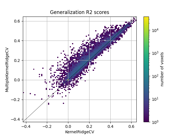
We see that the banded ridge model (MultipleKernelRidgeCV) outperforms
the ridge model (KernelRidegeCV). Indeed, banded ridge regression is able
to find the optimal scalings of each feature space, independently on each
voxel. Banded ridge regression is thus able to perform a soft selection
between the available feature spaces, based on the cross-validation
performances.
Plot the banded ridge split
On top of better prediction accuracy, banded ridge regression also gives a way to disentangle the contribution of the two feature spaces. To do so, we take the kernel weights and the ridge (dual) weights corresponding to each feature space, and use them to compute the prediction from each feature space separately.
Then, we use these split predictions to compute split \(\tilde{R}^2_i\) scores. These scores are corrected so that their sum is equal to the \(R^2\) score of the full prediction \(\hat{y}\).
from himalaya.scoring import r2_score_split

Y_test_pred_split = pipeline.predict(X_test, split=True)
split_scores_mask = r2_score_split(Y_test[:, mask], Y_test_pred_split)

print("(n_kernels, n_samples_test, n_voxels_mask) =", Y_test_pred_split.shape)
print("(n_kernels, n_voxels_mask) =", split_scores_mask.shape)

# extend to unfitted voxels
n_kernels = split_scores_mask.shape[0]
n_voxels = Y_train.shape[1]
split_scores = np.zeros((n_kernels, n_voxels))
split_scores[:, mask] = backend.to_numpy(split_scores_mask)
print("(n_kernels, n_voxels) =", split_scores.shape)
(n_kernels, n_samples_test, n_voxels_mask) = torch.Size([2, 270, 6849])
(n_kernels, n_voxels_mask) = torch.Size([2, 6849])
(n_kernels, n_voxels) = (2, 84038)
We can then plot the split scores on a flatmap with a 2D colormap.
from voxelwise_tutorials.viz import plot_2d_flatmap_from_mapper

mapper_file = os.path.join(directory, "mappers", f"{subject}_mappers.hdf")
ax = plot_2d_flatmap_from_mapper(split_scores[0], split_scores[1],
                                 mapper_file, vmin=0, vmax=0.25, vmin2=0,
                                 vmax2=0.5, label_1=feature_names[0],
                                 label_2=feature_names[1])
plt.show()
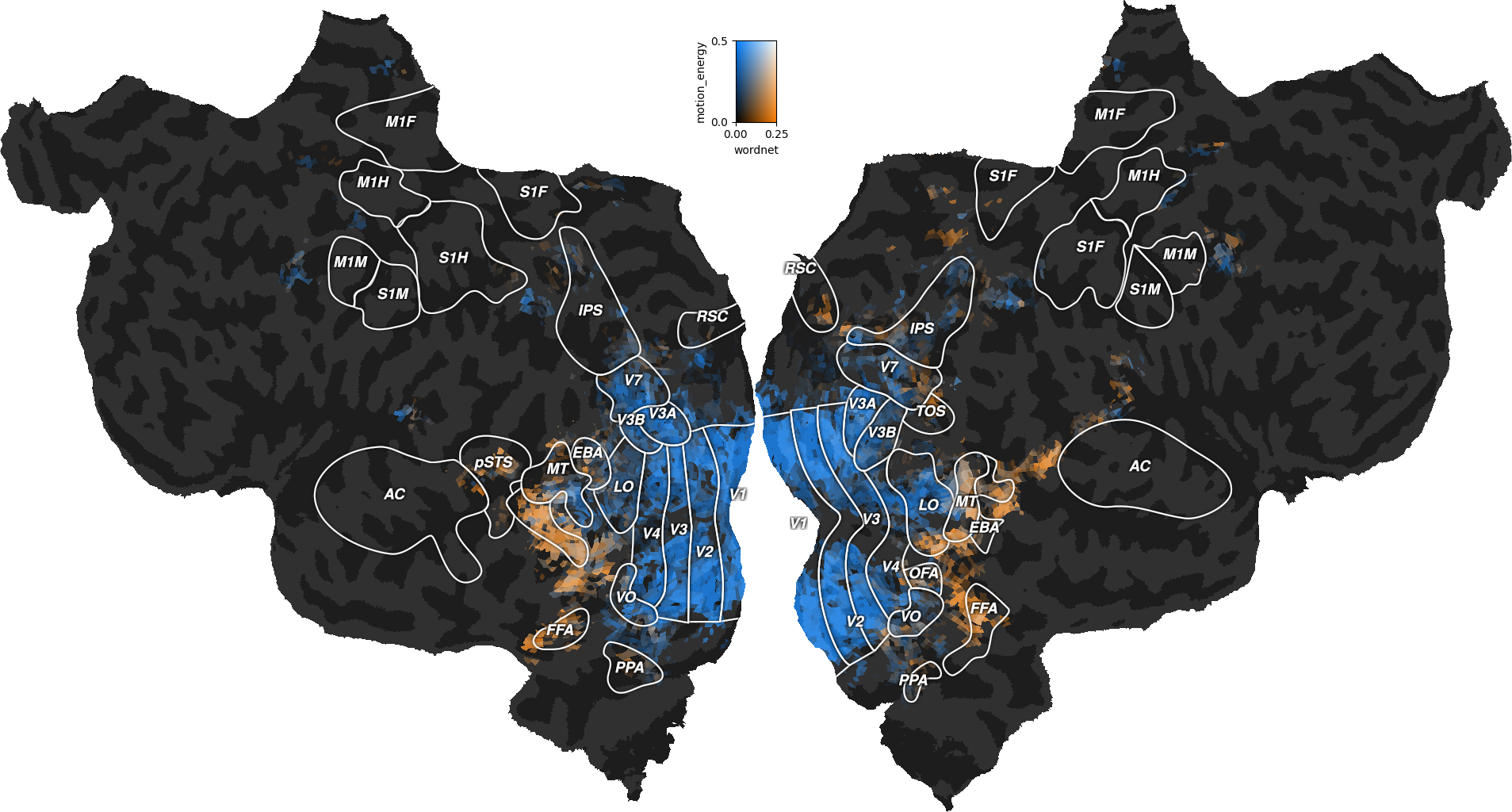
The blue regions are better predicted by the motion-energy features, the orange regions are better predicted by the wordnet features, and the white regions are well predicted by both feature spaces.
Compared to the last figure of the previous example, we see that most white regions have been replaced by either blue or orange regions. The banded ridge regression disentangled the two feature spaces in voxels where both feature spaces had good prediction accuracy (see previous example). For example, motion-energy features predict brain activity in early visual cortex, while wordnet features predict in semantic visual areas. For more discussions about these results, we refer the reader to the original publication [1].
References
Total running time of the script: (1 minutes 58.143 seconds)