Note
Go to the end to download the full example code
Fit a ridge model with motion energy features
In this example, we model the fMRI responses with motion-energy features extracted from the movie stimulus. The model is a regularized linear regression model.
This tutorial reproduces part of the analysis described in Nishimoto et al (2011) [1]. See this publication for more details about the experiment, the motion-energy features, along with more results and more discussions.
Motion-energy features: Motion-energy features result from filtering a video stimulus with spatio-temporal Gabor filters. A pyramid of filters is used to compute the motion-energy features at multiple spatial and temporal scales. Motion-energy features were introduced in [1].
Summary: As in the previous example, we first concatenate the features with multiple delays, to account for the slow hemodynamic response. A linear regression model then weights each delayed feature with a different weight, to build a predictive model of BOLD activity. Again, the linear regression is regularized to improve robustness to correlated features and to improve generalization. The optimal regularization hyperparameter is selected independently on each voxel over a grid-search with cross-validation. Finally, the model generalization performance is evaluated on a held-out test set, comparing the model predictions with the ground-truth fMRI responses.
Path of the data directory
from voxelwise_tutorials.io import get_data_home
directory = get_data_home(dataset="shortclips")
print(directory)
/home/jlg/mvdoc/voxelwise_tutorials_data/shortclips
# modify to use another subject
subject = "S01"
Load the data
We first load the fMRI responses.
import os
import numpy as np
from voxelwise_tutorials.io import load_hdf5_array

file_name = os.path.join(directory, "responses", f"{subject}_responses.hdf")
Y_train = load_hdf5_array(file_name, key="Y_train")
Y_test = load_hdf5_array(file_name, key="Y_test")

print("(n_samples_train, n_voxels) =", Y_train.shape)
print("(n_repeats, n_samples_test, n_voxels) =", Y_test.shape)
(n_samples_train, n_voxels) = (3600, 84038)
(n_repeats, n_samples_test, n_voxels) = (10, 270, 84038)
We average the test repeats, to remove the non-repeatable part of fMRI responses.
Y_test = Y_test.mean(0)

print("(n_samples_test, n_voxels) =", Y_test.shape)
(n_samples_test, n_voxels) = (270, 84038)
We fill potential NaN (not-a-number) values with zeros.
Y_train = np.nan_to_num(Y_train)
Y_test = np.nan_to_num(Y_test)
Then we load the precomputed “motion-energy” features.
feature_space = "motion_energy"
file_name = os.path.join(directory, "features", f"{feature_space}.hdf")
X_train = load_hdf5_array(file_name, key="X_train")
X_test = load_hdf5_array(file_name, key="X_test")

print("(n_samples_train, n_features) =", X_train.shape)
print("(n_samples_test, n_features) =", X_test.shape)
(n_samples_train, n_features) = (3600, 6555)
(n_samples_test, n_features) = (270, 6555)
Define the cross-validation scheme
We define the same leave-one-run-out cross-validation split as in the previous example.
from sklearn.model_selection import check_cv
from voxelwise_tutorials.utils import generate_leave_one_run_out

# indice of first sample of each run
run_onsets = load_hdf5_array(file_name, key="run_onsets")
print(run_onsets)
[ 0 300 600 900 1200 1500 1800 2100 2400 2700 3000 3300]
We define a cross-validation splitter, compatible with scikit-learn API.
n_samples_train = X_train.shape[0]
cv = generate_leave_one_run_out(n_samples_train, run_onsets)
cv = check_cv(cv)  # copy the cross-validation splitter into a reusable list
Define the model
We define the same model as in the previous example. See the previous example for more details about the model definition.
from sklearn.pipeline import make_pipeline
from sklearn.preprocessing import StandardScaler
from voxelwise_tutorials.delayer import Delayer
from himalaya.kernel_ridge import KernelRidgeCV
from himalaya.backend import set_backend
backend = set_backend("torch_cuda", on_error="warn")

X_train = X_train.astype("float32")
X_test = X_test.astype("float32")

alphas = np.logspace(1, 20, 20)

pipeline = make_pipeline(
    StandardScaler(with_mean=True, with_std=False),
    Delayer(delays=[1, 2, 3, 4]),
    KernelRidgeCV(
        alphas=alphas, cv=cv,
        solver_params=dict(n_targets_batch=500, n_alphas_batch=5,
                           n_targets_batch_refit=100)),
)
from sklearn import set_config
set_config(display='diagram')  # requires scikit-learn 0.23
pipeline
Fit the model
We fit on the train set, and score on the test set.
pipeline.fit(X_train, Y_train)

scores_motion_energy = pipeline.score(X_test, Y_test)
scores_motion_energy = backend.to_numpy(scores_motion_energy)

print("(n_voxels,) =", scores_motion_energy.shape)
(n_voxels,) = (84038,)
Plot the model performances
The performances are computed using the \(R^2\) scores.
import matplotlib.pyplot as plt
from voxelwise_tutorials.viz import plot_flatmap_from_mapper
mapper_file = os.path.join(directory, "mappers", f"{subject}_mappers.hdf")
ax = plot_flatmap_from_mapper(scores_motion_energy, mapper_file, vmin=0,
vmax=0.5)
plt.show()
The motion-energy features lead to large generalization scores in the early visual cortex (V1, V2, V3, …). For more discussions about these results, we refer the reader to the original publication [1].
Compare with the wordnet model
Interestingly, the motion-energy model performs well in different brain regions than the semantic “wordnet” model fitted in the previous example. To compare the two models, we first need to fit again the wordnet model.
feature_space = "wordnet"
file_name = os.path.join(directory, "features", f"{feature_space}.hdf")
X_train = load_hdf5_array(file_name, key="X_train")
X_test = load_hdf5_array(file_name, key="X_test")

X_train = X_train.astype("float32")
X_test = X_test.astype("float32")
We can create an unfitted copy of the pipeline with the clone function,
or simply call fit again if we do not need to reuse the previous model.
if False:
    from sklearn.base import clone
    pipeline_wordnet = clone(pipeline)
    pipeline_wordnet
pipeline.fit(X_train, Y_train)
scores_wordnet = pipeline.score(X_test, Y_test)
scores_wordnet = backend.to_numpy(scores_wordnet)
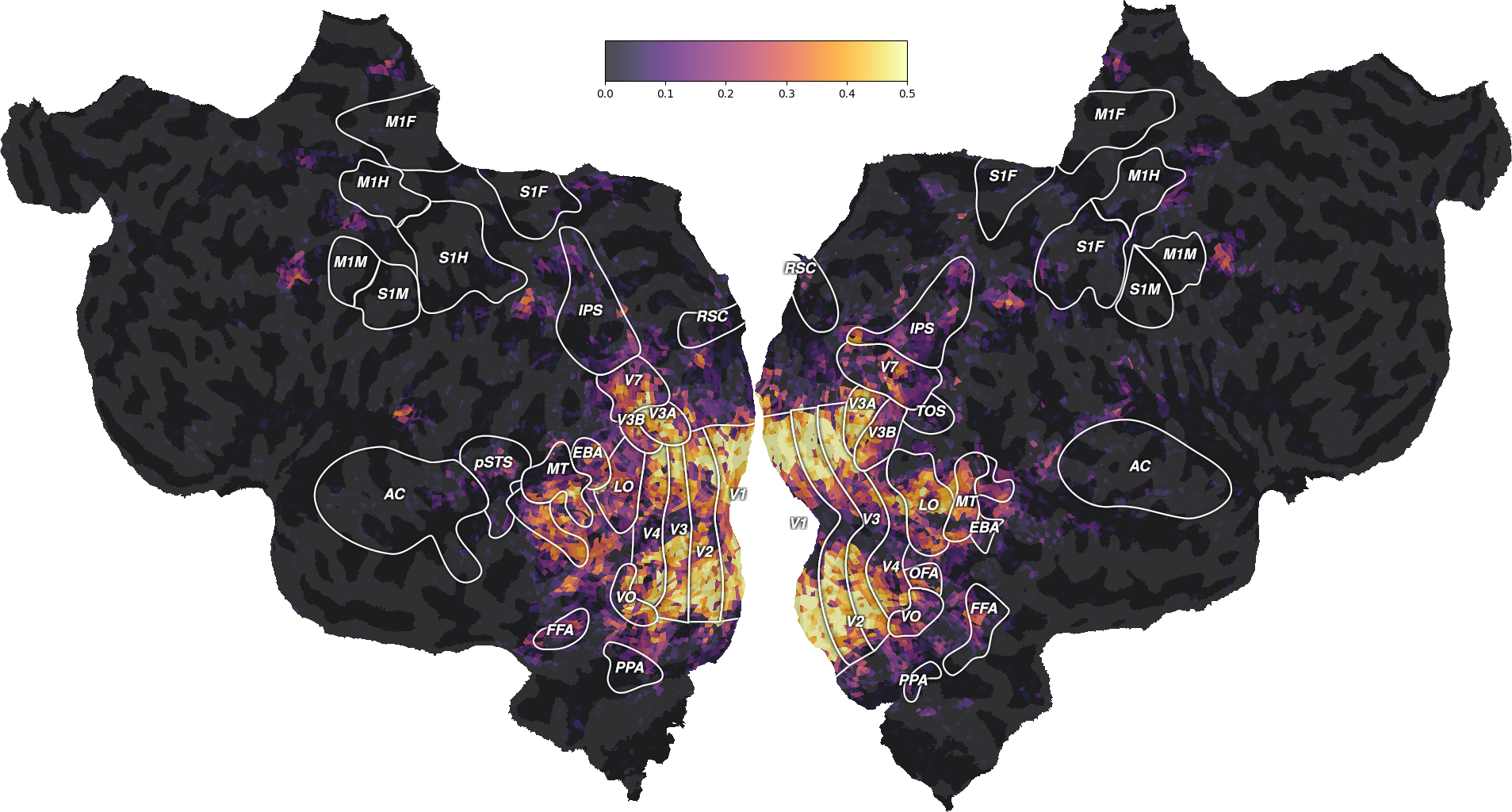
ax = plot_flatmap_from_mapper(scores_wordnet, mapper_file, vmin=0,
vmax=0.5)
plt.show()
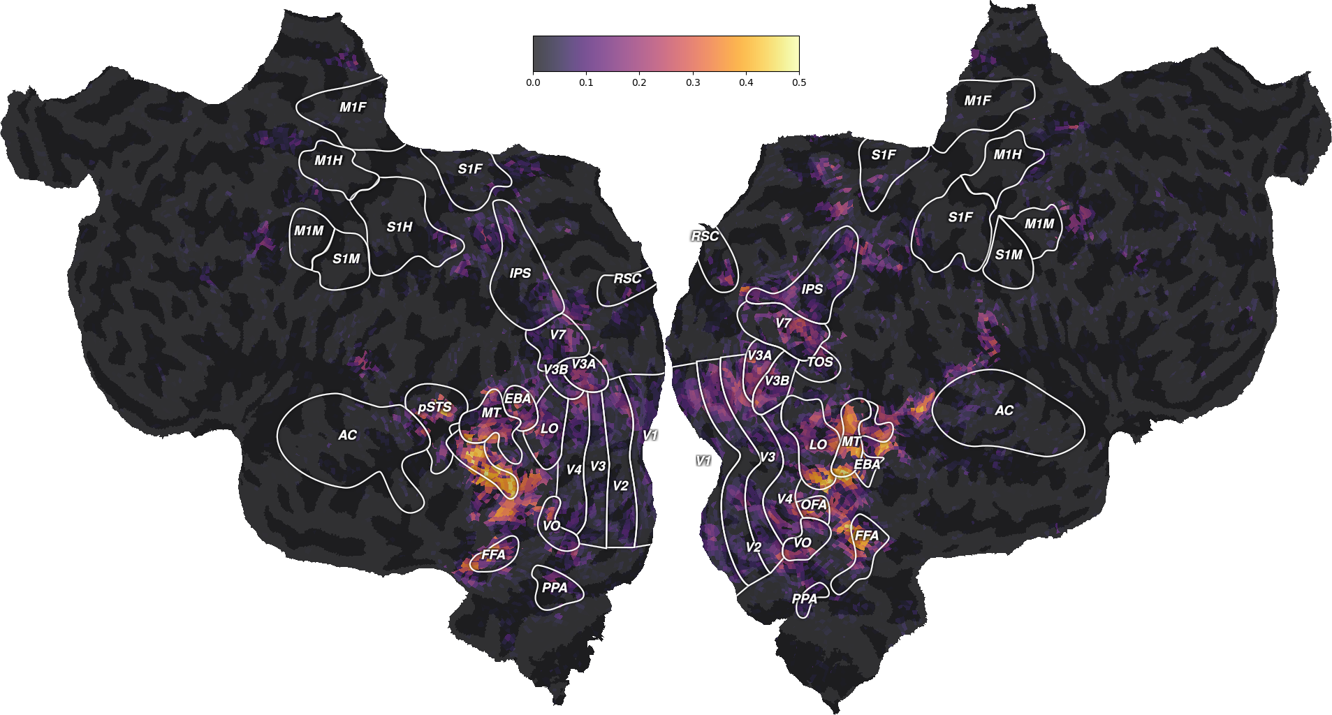
We can also plot the comparison of model prediction accuracies with a 2D histogram. All ~70k voxels are represented in this histogram, where the diagonal corresponds to identical prediction accuracy for both models. A distribution deviating from the diagonal means that one model has better predictive performance than the other.
from voxelwise_tutorials.viz import plot_hist2d

ax = plot_hist2d(scores_wordnet, scores_motion_energy)
ax.set(title='Generalization R2 scores', xlabel='semantic wordnet model',
       ylabel='motion energy model')
plt.show()
Interestingly, the well predicted voxels are different in the two models. To further describe these differences, we can plot both performances on the same flatmap, using a 2D colormap.
from voxelwise_tutorials.viz import plot_2d_flatmap_from_mapper

mapper_file = os.path.join(directory, "mappers", f"{subject}_mappers.hdf")
ax = plot_2d_flatmap_from_mapper(scores_wordnet, scores_motion_energy,
                                 mapper_file, vmin=0, vmax=0.25, vmin2=0,
                                 vmax2=0.5, label_1="wordnet",
                                 label_2="motion energy")
plt.show()
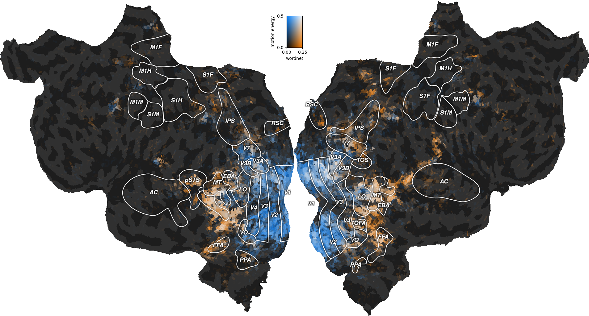
The blue regions are well predicted by the motion-energy features, the orange regions are well predicted by the wordnet features, and the white regions are well predicted by both feature spaces.
A large part of the visual semantic areas are not only well predicted by the wordnet features, but also by the motion-energy features, as indicated by the white color. Since these two features spaces encode quite different information, two interpretations are possible. In the first interpretation, the two feature spaces encode complementary information, and could be used jointly to further increase the generalization performance. In the second interpretation, both feature spaces encode the same information, because of spurious stimulus correlations. For example, imagine that the visual stimulus contained faces that appeared consistetly in the same portion of the visual field. In this case, position in the visual field would be perfectly correlated with the “face” semantic category. Thus, motion-energy features could predict responses in face-responsive areas without encoding any semantic information.
To better disentangle the two feature spaces, we developed a joint model called banded ridge regression [2], which fits multiple feature spaces simultaneously with optimal regularization for each feature space. This model is described in the next example.
References
Total running time of the script: (0 minutes 58.974 seconds)