Spatial components of the motion energy filters

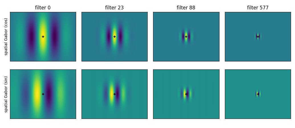
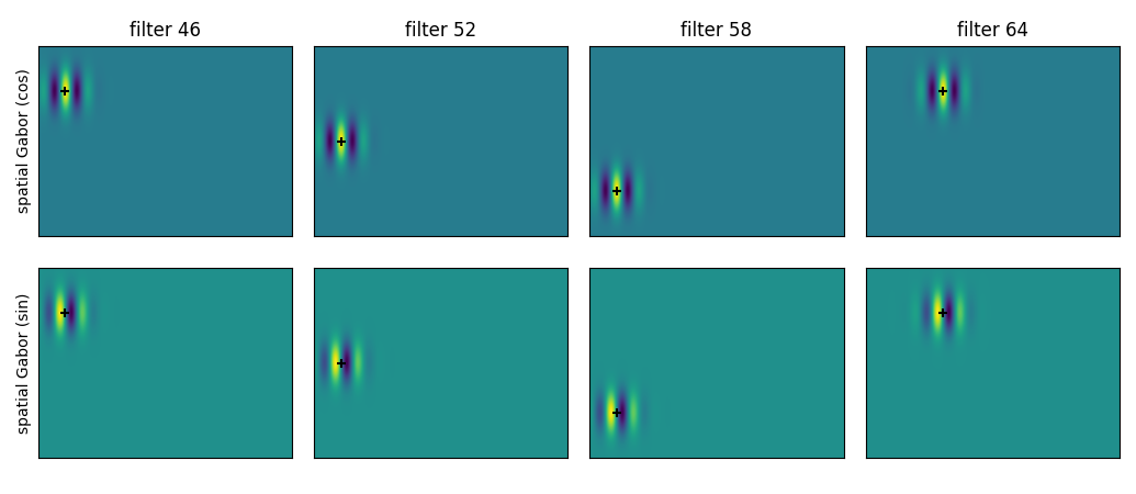
This example shows the spatial components of the spatio-temporal filters used in motion energy features. It does not show the temporal components, since this gallery does not support animation. To visualize the filters with their temporal components, you can use moten.viz.plot_3dgabor(). Here we demonstrate how the spatial filters vary in term of spatial frequencies, locations, and directions.

First, let’s define a motion energy pyramid, using MotionEnergyPyramid. It defines a set of spatio-temporal Gabor filters.

import moten
pyramid = moten.pyramids.MotionEnergyPyramid(stimulus_vhsize=(300, 400),
                                             stimulus_fps=25)

Then, we define a plotting function, to show the spatial part of these spatio-temporal Gabor filters.

import matplotlib.pyplot as plt  # noqa


def plot_spatial_gabors(pyramid, indices):
    """Plot the two quadrature spatial components of a list of Gabor filters.

    Note this only show the spatial components of the spatio-temporal filters.

    Parameters
    ----------
    pyramid : moten.pyramid.MotionEnergyPyramid instance
    indices : list of int
    """
    vdim = pyramid.definition['vdim']

    size = 0.6
    fig, axs = plt.subplots(
        2, len(indices), figsize=((len(indices) * 4.25 + 0.25) * size,
                                  7.5 * size), squeeze=False,
        sharex=True, sharey=True)

    axs.T[0][0].set_ylabel('spatial Gabor (cos)')
    axs.T[0][1].set_ylabel('spatial Gabor (sin)')

    for ii, axs_ in zip(indices, axs.T):

        spatial_sin, spatial_cos = pyramid.get_filter_spatial_quadrature(ii)
        axs_[0].imshow(spatial_cos, aspect='equal')
        axs_[1].imshow(spatial_sin, aspect='equal')
        axs_[0].set_title('filter %d' % ii)

        gabor = pyramid.filters[ii]
        for ax in axs_:
            ax.scatter(gabor['centerh'] * vdim, gabor['centerv'] * vdim,
                       color='k', marker='+')
            ax.set_xticks([])
            ax.set_yticks([])

    plt.tight_layout()

Different spatial frequencies

plot_spatial_gabors(pyramid, [0, 23, 88, 577])

Different locations

plot_spatial_gabors(pyramid, [46, 52, 58, 64])

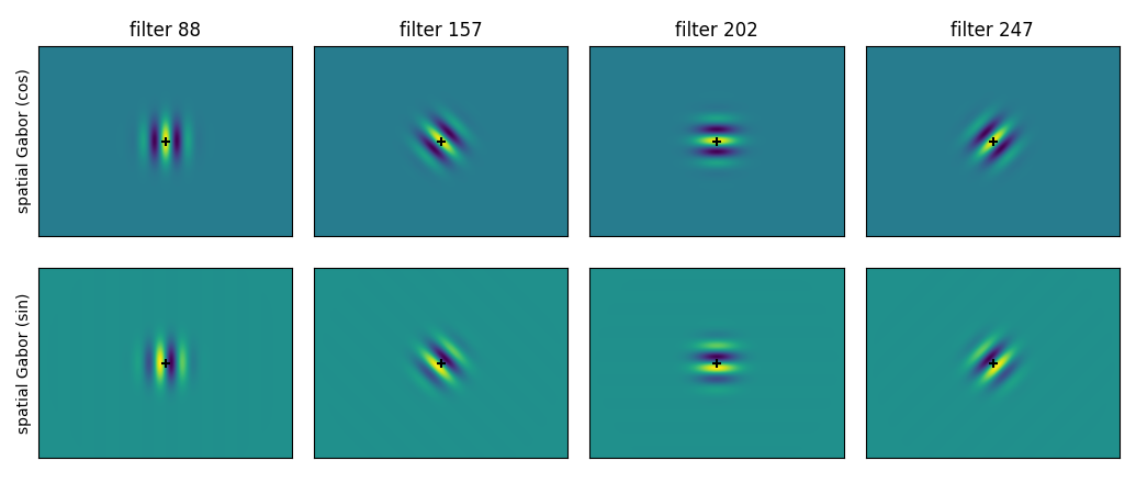
Different directions

plot_spatial_gabors(pyramid, [88, 157, 202, 247])